Masking attention weights in PyTorch
Attention has become ubiquitous in sequence learning tasks such as machine translation. We most often have to deal with variable length sequences but we require each sequence in the same batch (or the same dataset) to be equal in length if we want to represent them as a single tensor. Padding shorter sentences to the same length as the longest one in the batch is the most common solution for this problem.
There are many formulations for attention but they share a common goal: predict a probability distribution called attention weights over the sequence elements. The most common way of ensure that the weights are a valid probability distribution (all values are non-negative and they sum to 1) is to use the softmax function, defined for each sequence element as:
where $N$ is the length of the sequence and $exp$ is the exponential function.
Our working example is going to be a toy dataset of 4 sequences and a separate vector that contains the length of each sequence. We align the sequences to the left and pad them on the right.
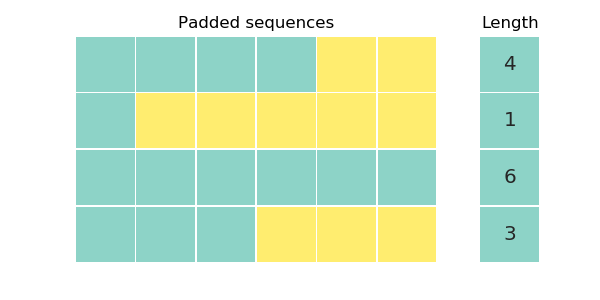
When using padding we require attention to focus solely on the valid symbols and assing zero weight to pad symbols since they do not carry useful information. Our final goal is to assign non-zero attention weights to real symbols (in blue) and zero weights to pad symbols (in yellow). In the example, pad symbols have zero weights and all rows sum to one (aside from rounding errors).
Setting the weight of pad symbols to zero after softmax breaks the probability distribution, rows will no longer sum to one, so we need to ensure that the output of softmax is zero for these values by setting them to negative infinity beforehand. PyTorch and NumPy allow setting certain elements of a tensor using boolean masks. Mask are the same size as the tensor being masked and only those elements are updated where the mask value is true:
X = torch.arange(12).view(4, 3)
mask = torch.zeros((4, 3), dtype=torch.uint8)  # or dtype=torch.ByteTensor
mask[0, 0] = 1
mask[1, 1] = 1
mask[3, 2] = 1
X[mask] = 100
print(X)

> tensor([[100,   1,   2],
          [  3, 100,   5],
          [  6,   7,   8],
          [  9,  10, 100]])
Masks can also be inverted with the ~ operator:
X = torch.arange(12).view(4, 3)
X[~mask] = 100
print(X)

> tensor([[  0, 100, 100],
          [100,   4, 100],
          [100, 100, 100],
          [100, 100,  11]])
Let’s define our dataset as tensors:
# generating the actual toy example
np.random.seed(1)
X = np.random.random(data.shape).round(1) * 2 + 3
X = torch.from_numpy(X)
X_len = torch.LongTensor([4, 1, 6, 3])  # length of each sequence
Now all we need to do is create a mask with true values in place of real values and zeros in pad values and use that mask before softmax. We apply a little broadcasting trick for this:
maxlen = X.size(1)
mask = torch.arange(maxlen)[None, :] < X_len[:, None]
print(mask)
> tensor([[1, 1, 1, 1, 0, 0],
          [1, 1, 1, 1, 1, 1],
          [1, 0, 0, 0, 0, 0],
          [1, 1, 1, 1, 1, 1]], dtype=torch.uint8)
None indices create dummy dimensions which can repeat the real data as many
times as necessary for the operation. The left operand of < is a sequence of
index values $i=0, \dots , N-1$. The right operand is the length vector itself.
Wherever the index is smaller than the sequence length corresponding to that
row, we have a real element. We are broadcasting a row vector (indices) with a
column vector (length) and we want the index vector repeated for each row (4
times) and the length vector repeated for each column (10 times), which we can
do by adding a dummy dimension as the first dimension to the left operand and
as the second dimension to the right operand. None are replaced with 4 and 10
repetitions in this case. You can read more about PyTorch broadcasting
here.
A less concise but perhaps more readable way to create the mask is to manually expand both tensors:
maxlen = X.size(1)
idx = torch.arange(maxlen).unsqueeze(0).expand(X.size())
print(idx)
len_expanded = X_len.unsqueeze(1).expand(X.size())
print(len_expanded)
mask = idx < len_expanded
print(mask)

> tensor([[0, 1, 2, 3, 4, 5],
          [0, 1, 2, 3, 4, 5],
          [0, 1, 2, 3, 4, 5],
          [0, 1, 2, 3, 4, 5]])
> tensor([[4, 4, 4, 4, 4, 4],
          [1, 1, 1, 1, 1, 1],
          [6, 6, 6, 6, 6, 6],
          [3, 3, 3, 3, 3, 3]])
> tensor([[1, 1, 1, 1, 0, 0],
          [1, 0, 0, 0, 0, 0],
          [1, 1, 1, 1, 1, 1],
          [1, 1, 1, 0, 0, 0]], dtype=torch.uint8)
The former is about 15% faster than the latter when tested on CPU.
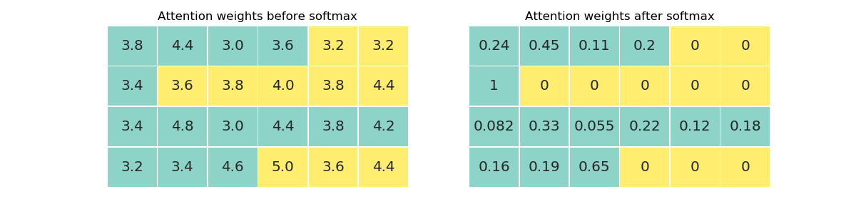
Using inverse masking, we set the pad values’ attention weights to negative infinity and then call softmax:
X[~mask] = float('-inf')
print(X)
print(torch.softmax(x, dim=1))

> tensor([[3.8000, 4.4000, 3.0000, 3.6000,   -inf,   -inf],
          [3.4000,   -inf,   -inf,   -inf,   -inf,   -inf],
          [3.4000, 4.8000, 3.0000, 4.4000, 3.8000, 4.2000],
          [3.2000, 3.4000, 4.6000,   -inf,   -inf,   -inf]], dtype=torch.float64)

> tensor([[0.2445, 0.4455, 0.1099, 0.2002, 0.0000, 0.0000],
          [1.0000, 0.0000, 0.0000, 0.0000, 0.0000, 0.0000],
          [0.0822, 0.3335, 0.0551, 0.2235, 0.1227, 0.1830],
          [0.1593, 0.1946, 0.6461, 0.0000, 0.0000, 0.0000]], dtype=torch.float64)
The jupyter notebook used for the examples along with all visualization is available here.