Exploring BERT's Vocabulary
Deep contextualized word representations have taken word representation to the next level by assigning word vectors to words in context - typically a sentence - instead of assigning a vector to each word type. ELMO and BERT are the most popular and successful examples of these embeddings. The authors of BERT released several versions of BERT pretrained on massive amounts of data, including a multilingual version which supports 104 languages in a single model.
Multilingual BERT Vocabulary
I was admittedly intrigued by the idea of a single model for 104 languages with
a large shared vocabulary. The vocabulary is 119,547 WordPiece model, and the
input is tokenized into word pieces (also known as subwords) so that each
word piece is an element of the dictionary. Non-word-initial units are prefixed
with ## as a continuation symbol except for Chinese characters which are
surrounded by spaces before any tokenization takes place. The tokenizer favors
longer word pieces with a de facto character-level model as a fallback as every
character is part of the vocabulary as a possible word piece. An example of
such tokenization using Hugging Face’s PyTorch implementation of
BERT looks like this:
tokenizer = BertTokenizer.from_pretrained(
    "bert-base-multilingual-cased", do_lower_case=False)
tokenizer.tokenize("Elvégezhetitek")

['El', '##vé', '##ge', '##zhet', '##ite', '##k']
This segmentation is purely frequency based and it is very different from what a true morphological segmenter would output (El-végez-het-itek). This example is certainly longer than an average Hungarian word and the average word is not tokenized this aggressively but BERT does produce a large number of word pieces for certain languages. I will examine this closer in this post.
The first 106 symbols are reserved for constants like PAD and UNK and
unused placeholders for application specific symbols. 36.5% of the vocabulary
are non-initial word pieces. The alphabet consists of 9,997 unique characters
that are defined as word-initial (C) and continuation symbols (##C), which
together make up 19,994 word pieces. The rest are multicharacter word
pieces of various length.
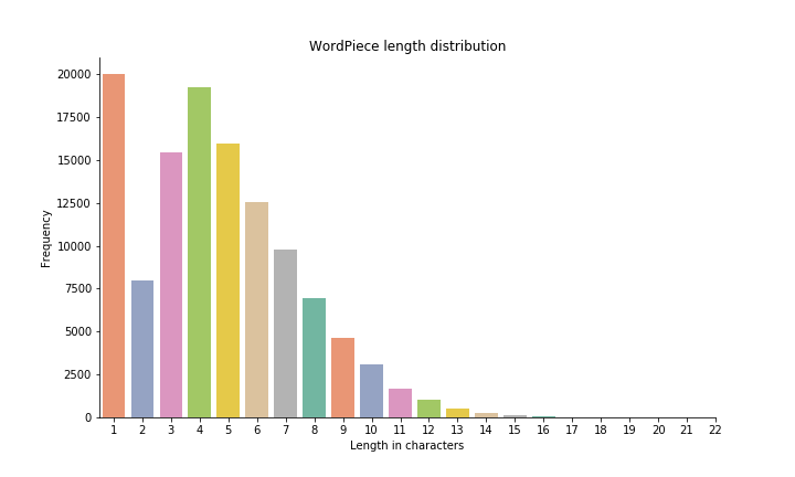
As the length distribution shows single character symbols are the largest group with a sharp drop after that and a somewhat surprising second peak at 4-character symbols. Most units are very short with a few exceptions over 20 characters. The list of the 20 longest symbols features many German compounds and other long words frequent in Wikipedia:
| Token | Length | Token | Length |
|---|---|---|---|
| bewerkingsgeschiedenis | 22 | Auseinandersetzungen | 20 |
| ուսումնասիրությունների | 22 | தொகுக்கப்பட்டுள்ளது | 19 |
| Territorialgeschichte | 21 | delstatshuvudstaden | 19 |
| Europameisterschaften | 21 | Bevölkerungsstandes | 19 |
| huvudavrinningsområde | 21 | Nationalsozialisten | 19 |
| தேர்ந்தெடுக்கின்றனர் | 20 | Weltmeisterschaften | 19 |
| Rechtswissenschaften | 20 | delavrinningsområde | 19 |
| eenoogkreeftjessoort | 20 | bevolkingsdichtheid | 19 |
| Årsmedeltemperaturen | 20 | Nationalsozialismus | 19 |
| நிர்வகிக்கப்படுகிறது | 20 | Europameisterschaft | 19 |
The vocabulary was created using the top 100 Wikipedia dumps. The authors oversampled small Wikipedias so we should see many non-English looking word pieces in the vocabulary. To test this, I used the predefined ranges of Unicode code points obtained from here. If you are unfamiliar with Unicode, I highly recommend Joel Spolsky’s amazing introduction. I grouped the ranges into overlapping macro categories such as ASCII, Latin (includes diacritics), CJK (Chinese, Japanese, Korean), CJK+Kana (CJK, Hiragana, Katakana), Cyrillic, Korean Hangul, Indian (various alphabets used mainly in India) etc. The exact mapping is available here.
We can match ranges of Unicode character with Python regular expressions like this:
# Japanese Hiragana Unicode range
start = 0x3040
end = 0x309f

# match one or more Hiragana characters
pattern = r'[\U{0:08X}-\U{1:08X}]+'.format(start, end)
print(pattern)
hiragana_re = re.compile(pattern)
print(hiragana_re.match("abc"))
print(hiragana_re.match("ひらがな"))

-------
Output:
[\U00003040-\U0000309F]+
None
<re.Match object; span=(0, 4), match='ひらがな'>
we can extend this regular expression to allow digits but require at least one
character from the Unicode range. The abstract regex looks like this [Hiragana
or digit]*[Hiragana]+[Hiragana or digit]*, it accepts one or more
([Hiragana]+) prefixed and/or suffixed by zero or more Hiragana/digits
([Hiragana or digit]*).
start = 0x3040
end = 0x309f

hiragana_re = re.compile(r'^[\U{0:08X}-\U{1:08X}\d]*'
                         r'[\U{0:08X}-\U{1:08X}]+'
                         r'[\U{0:08X}-\U{1:08}\d]*$'.format(start, end))

print(hiragana_re.match("a"))
print(hiragana_re.match("1"))
print(hiragana_re.match("お1"))
print(hiragana_re.match("1お"))
print(hiragana_re.match("おお12お"))
print(hiragana_re.match("ひらがな"))

-------
Output:
None
None
<re.Match object; span=(0, 2), match='お1'>
<re.Match object; span=(0, 2), match='1お'>
<re.Match object; span=(0, 5), match='おお12お'>
<re.Match object; span=(0, 4), match='ひらがな'>
I defined a regular expression for each macro category. A word piece belongs to the category if all of its characters fall into the category or are digits. Pure digits are excluded from non-Latin or ASCII. It turns out that 78% of the word pieces fall into the Latin category, most of them are pure ASCII (77% of all pieces). The rest of the categories are much smaller, probably due to their respective Wikipedias being much smaller than that of the European languages. This table lists how many word pieces were matched by each category:
| Script | Sum | % |
|---|---|---|
| Latin | 93495 | 78.21 |
| ASCII | 92327 | 77.23 |
| CJK+kana | 14932 | 12.49 |
| Cyrillic | 13782 | 11.53 |
| CJK | 13601 | 11.38 |
| Indian | 6545 | 5.47 |
| Arabic | 4873 | 4.08 |
| Korean | 3273 | 2.74 |
| Hebrew | 2482 | 2.08 |
| Greek | 1566 | 1.31 |
| Kana | 1331 | 1.11 |
| Armenian | 1236 | 1.03 |
| Georgian | 705 | 0.59 |
| Misc | 639 | 0.53 |
| Thai | 370 | 0.31 |
| Myanmar | 271 | 0.23 |
| Tibetan | 40 | 0.03 |
| Mongolian | 4 | 0.0 |
Tokenizing Universal Dependency Treebanks
Universal Dependencies (UD) is a framework for
grammatical annotation with treebanks available in more than 70 languages, 54
overlapping with BERT’s language list. The smallest treebanks are Tagalog (55
sentences) and Yoruba (100 sentences), while the largest ones are Czech
(127,507) and Russian (69,683). I tokenized each treebank with BertTokenizer
and compared the tokenization with the gold standard tokenization. The input to
BertTokenizer was the full text form of the sentence.
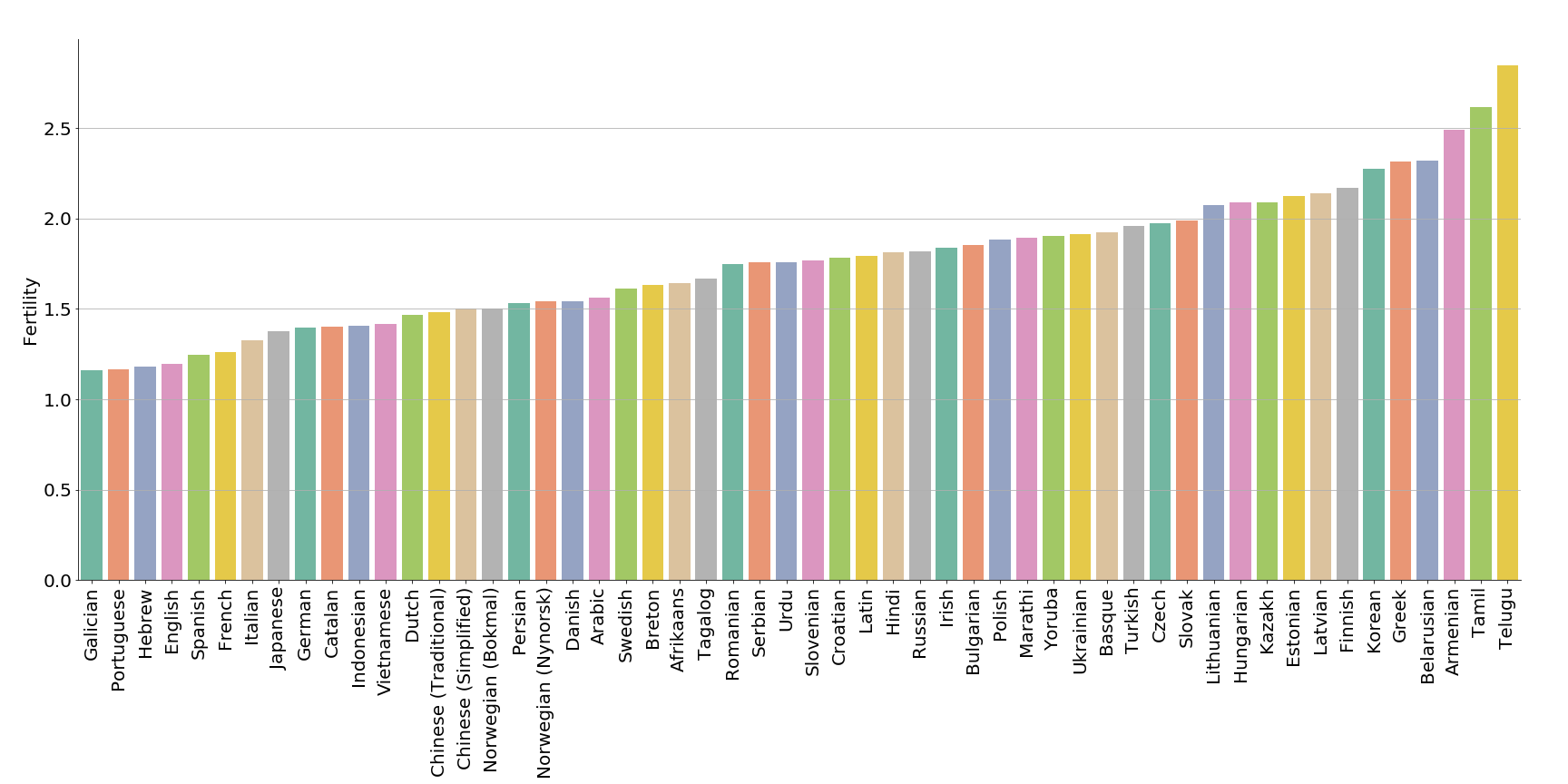
Let’s define fertility, borrowed from statistical machine translation, as the
average number of BERT word pieces corresponding with a single real token. The
example ['El', '##vé', '##ge', '##zhet', '##ite', '##k'] has a fertility 6,
but we can expect lower values on average. Fertility would be 1 if all tokens
were in BERT’s vocabulary. As illustrated in this plot, BERT has the lowest
fertility in Galician (1.16) and the highest in Telugu (2.85). It should be
noted UD Treebanks differ in tokenization, for example Japanese tokenizes
inflections as separate tokens, while Korean does not, even though their
morphology shares many similarities. More aggressive tokenization results in
lower fertility values.
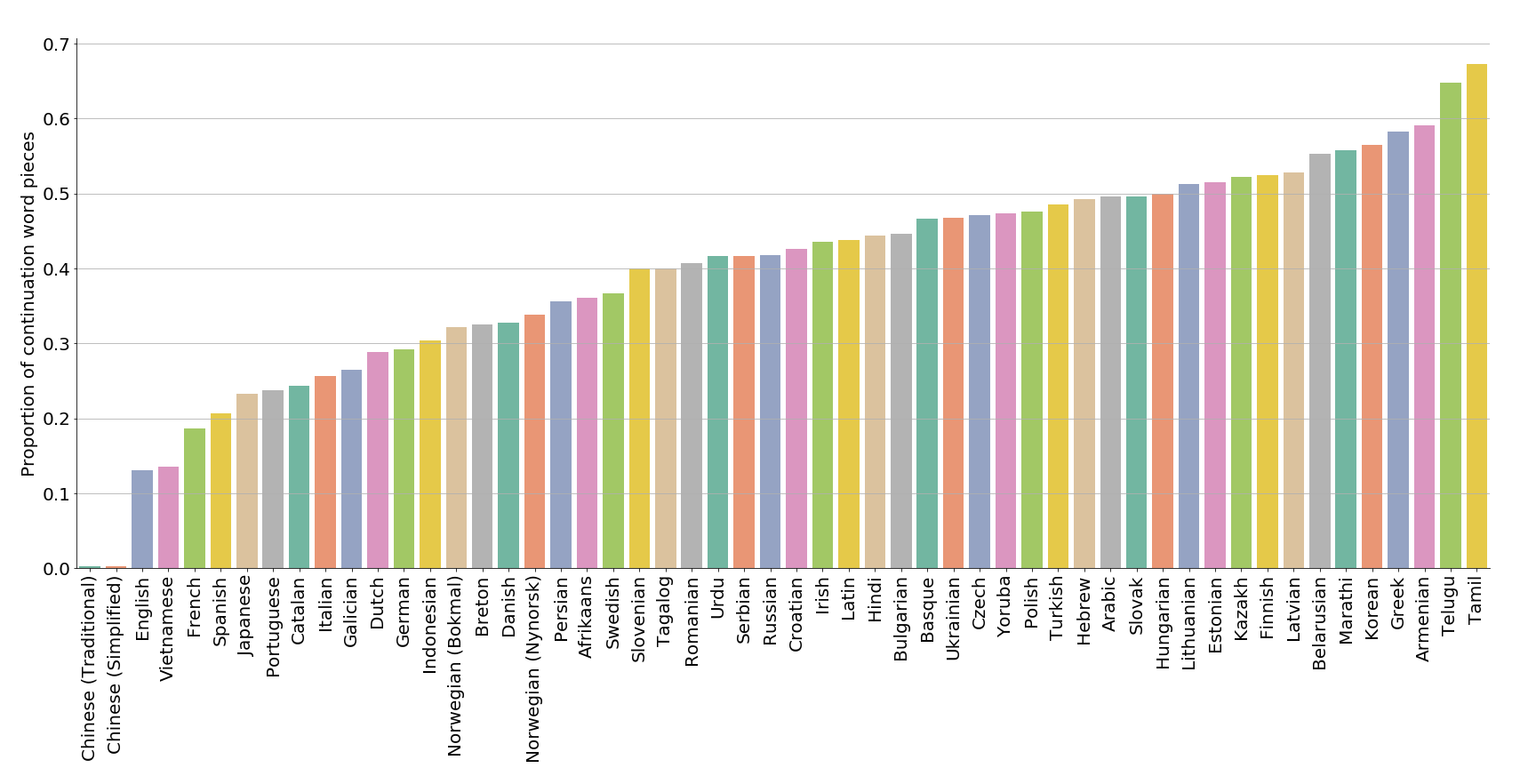
Examining the proportion of continuation word pieces shows us a different picture. Since Chinese characters are presegmented, there are barely any continuation word pieces (0.2%), with English (13.1%) and Vietnamese (13.5%) following. The highest proportion of continuation word pieces can be found in Tamil (67.3%) and Telugu (64.7%).
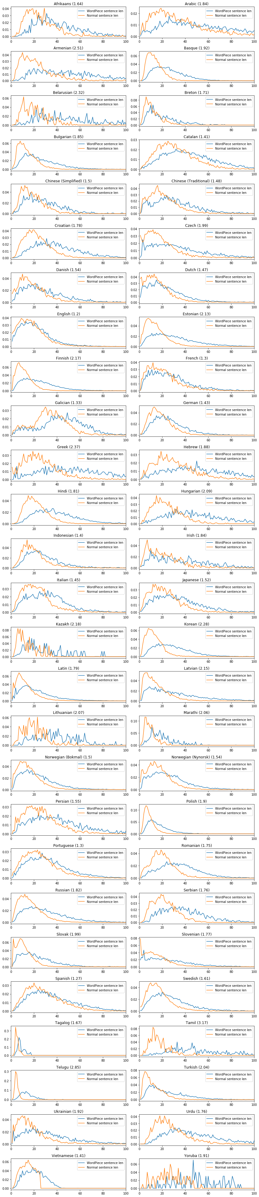
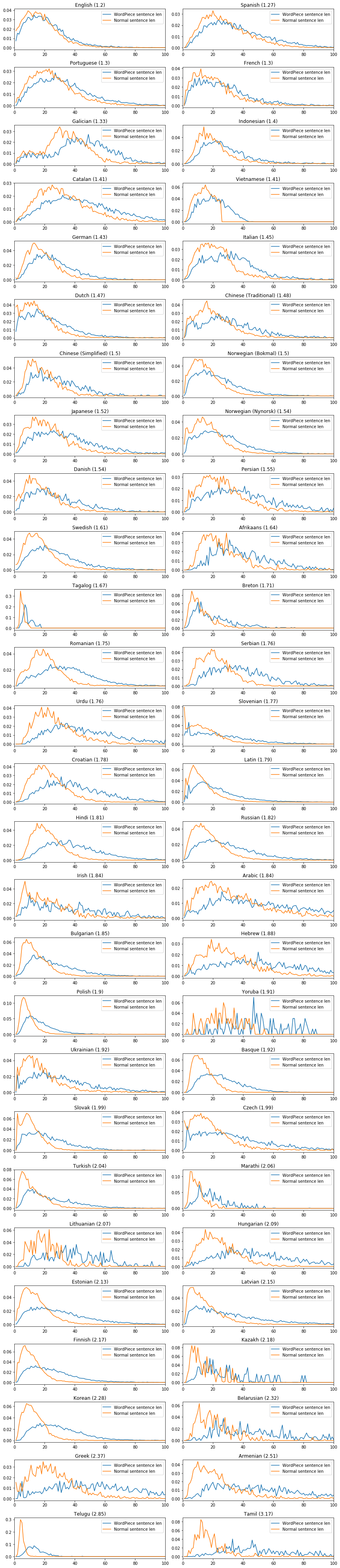
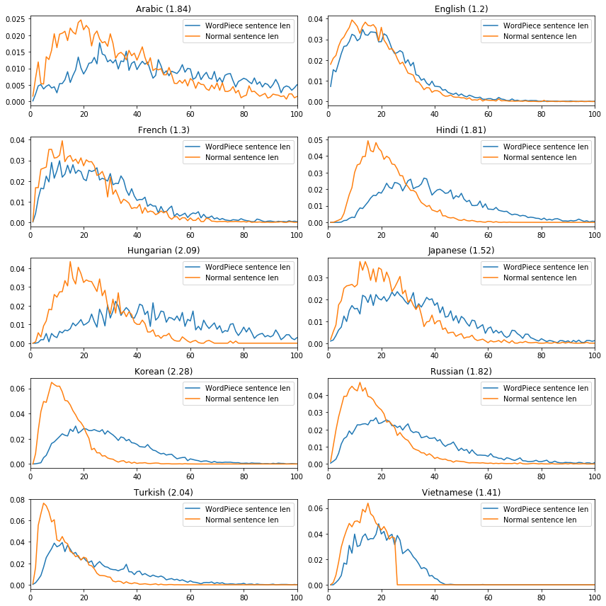
Similar trends can be found in the sentence length distribution defined as the number of tokens in a sentence. Here is a comparison for a few cherrypicked languages. The x-axes represent the sentence length in tokens and the y-axes are the proportion of sentences of certain length. Fertility values are listed in parentheses above each plot. The full list in alphabetical order is available here, and sorted by fertility here.
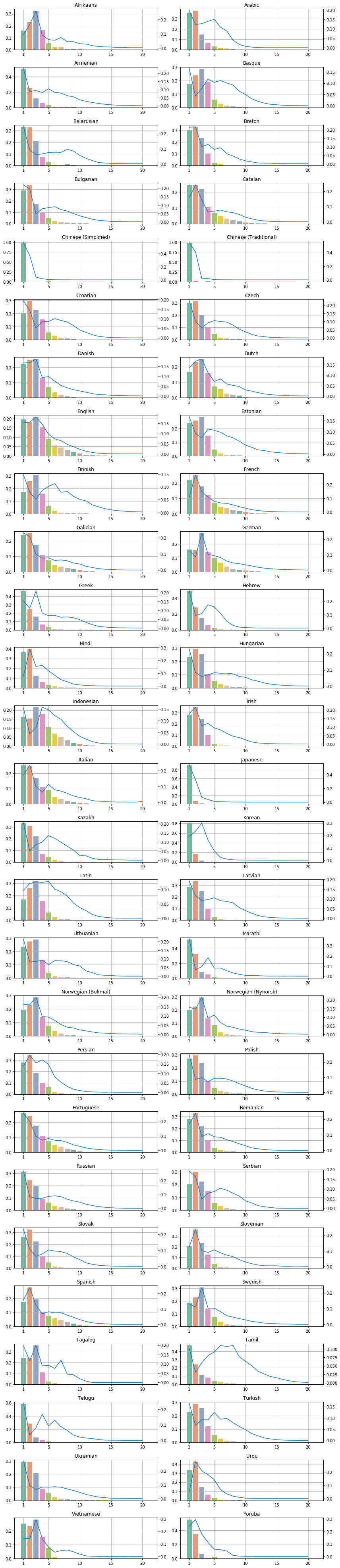
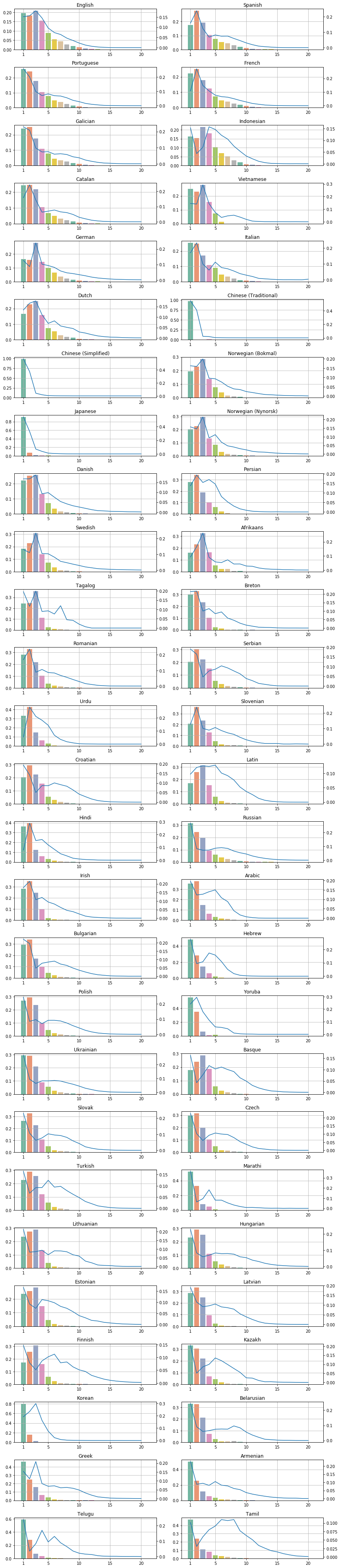
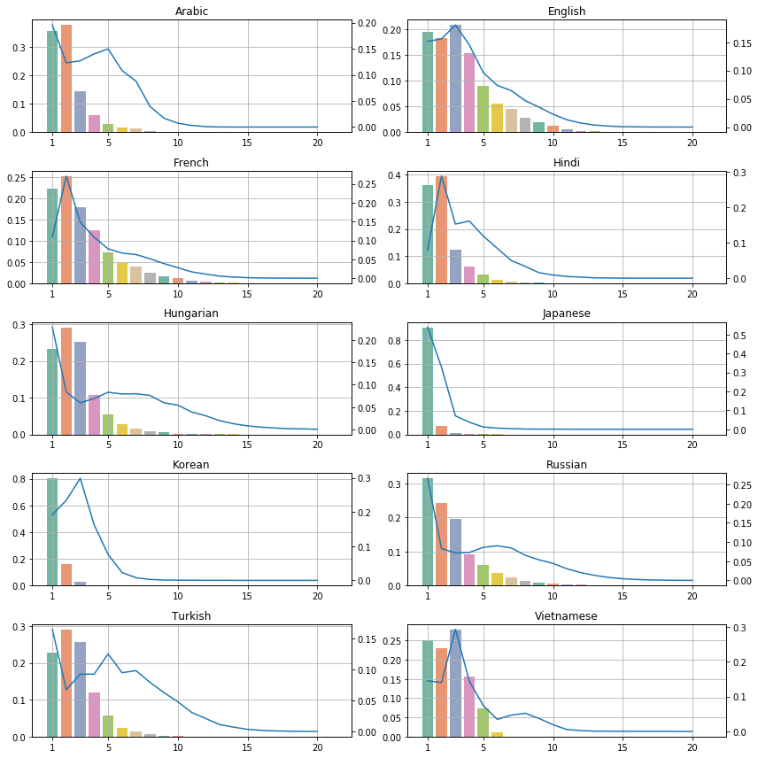
Finally the prettiest plots show how BERT affects the distribution of token length in the same languages. The bars represent the ratio of N-long BERT word pieces, while the blue curves show the original token length distribution. The y-axes are scaled differently, the bars’ scale is shown on the left, and the curve’s scale is shown on the right side of each plot. The full list in alphabetical order is available here, and sorted by fertility here.
Conclusion
I explored BERT’s multilingual vocabulary by itself and through its tokenization on 54 languages that have UD treebanks. I found that the majority of elements in BERT’s vocabulary are that of the European languages, most of them pure ASCII. Examining the output of BERT tokenizer confirmed that the tokenizer keeps English mostly intact while it may generate different token distributions in morphologically rich languages. The degree of how much this tokenization resembles a morphological segmentation remains to be explored.
Code
The script used to extract BERT and UD stats can be found here. This notebook contains all code used to generate the plots. Raw statistics are available as TSV in the same directory.
Acknowledgment
I would like to thank Ofir Press and my Hungarian colleagues for feedback on earlier drafts of this article.